The regression bootstrap tool performs a bootstrapped estimate of a confidence interval for the least squares regression slope relating two variables. From the Data menu select Built-in for a dataset from the archive or Import… to use your own data. Imported data should be in tab-delimited text format with variable names in the first row.
You will then see the first row of the data and a drop-down menu from which to choose the columns of your data table you wish to relate. When you select the columns, the tool will make a scatterplot of the data and show a least squares regression line. The means of the two variables and the slope of the line are shown to the right of the scatterplot.
To choose different columns, select the Change Variable command from the Data menu.
Now specify the number of bootstrap samples to draw.
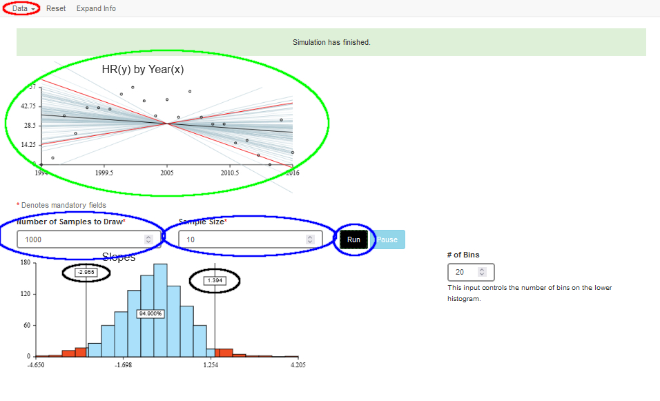
Click the Run button to perform the bootstrap. As a bootstrap sample is drawn, the corresponding points highlight on the scatterplot and the least squares slope corresponding to those points is drawn on the plot. The scatterplot shows a “sheaf” of regression lines fit for each bootstrap sample. The lower graph is a histogram of the slopes of the bootstrap samples as they are drawn. It also shows limits on a middle portion of those means. You can drag the flags at the edges to see how wide an interval is needed to find a bootstrap confidence interval for the slope. When you do this, the scatterplot of the data shows the corresponding slope limits with red lines.
Technical note: There are other ways to bootstrap for regression slopes. This is the simplest, but it may not yield the narrowest confidence intervals. Consult more technical sources for details.
- Use the Data menu to enter a data set (circled in Red)
- Use built-in data (includes data for exercises in Intro Stats)
- Import data from a tab-delimited text file
- Paste data from the clipboard
- Select X and Y variables from the dataset
- The scatterplot will plot them (circled in Green)
- Choose a Sample size and Number of Samples. Click Run (circled in Blue)
- Selected cases highlight in the scatterplot and a regression for those cases is shown
- Slopes accumulate in the histogram
- Drag the limits to identify a central region (circled in Black). Observe the corresponding limits in the scatterplot